To explain this section we will start with a practical case: Let’s take the movement of the EURUSD as an example and choose one hour as the calculation period.
We must keep in mind that we could have taken any period to do the example (one minute, 5 minutes, one week, etc.).
We take as the price the average between the ask price and the bid price.
Let’s calculate the hourly variation in the movement of the EURUSD on any given day.
| Variation in hours | |||||
| Hour | Ask | Bid | Price | In price | In Pips |
| 1:00:00 | 1,08117 | 1,08115 | 1,08116 | 0,00000 | 0 |
| 2:00:00 | 1,08215 | 1,08212 | 1,08214 | 0,00097 | 97,5 |
| 3:00:00 | 1,08187 | 1,08184 | 1,08186 | -0,00028 | -28 |
| 4:00:00 | 1,08171 | 1,08170 | 1,08171 | -0,00015 | -15 |
| 5:00:00 | 1,08140 | 1,08137 | 1,08139 | -0,00032 | -32 |
| 6:00:00 | 1,08124 | 1,08122 | 1,08123 | -0,00015 | -15,5 |
| 7:00:00 | 1,08091 | 1,08091 | 1,08091 | -0,00032 | -32 |
| 8:00:00 | 1,08127 | 1,08126 | 1,08127 | 0,00036 | 35,5 |
| 9:00:00 | 1,08112 | 1,08110 | 1,08111 | -0,00016 | -15,5 |
| 10:00:00 | 1,08162 | 1,08156 | 1,08159 | 0,00048 | 48 |
| 11:00:00 | 1,08108 | 1,08105 | 1,08107 | -0,00052 | -52,5 |
| 12:00:00 | 1,08189 | 1,08187 | 1,08188 | 0,00081 | 81,5 |
| 13:00:00 | 1,08132 | 1,08129 | 1,08131 | -0,00057 | -57,5 |
| 14:00:00 | 1,08129 | 1,08127 | 1,08128 | -0,00002 | -2,5 |
| 15:00:00 | 1,08221 | 1,08199 | 1,08210 | 0,00082 | 82 |
| 16:00:00 | 1,08356 | 1,08354 | 1,08355 | 0,00145 | 145 |
| 17:00:00 | 1,08308 | 1,08306 | 1,08307 | -0,00048 | -48 |
| 18:00:00 | 1,08379 | 1,08376 | 1,08378 | 0,00071 | 70,5 |
| 19:00:00 | 1,08408 | 1,08406 | 1,08407 | 0,00029 | 29,5 |
| 20:00:00 | 1,08415 | 1,08412 | 1,08414 | 0,00006 | 6,5 |
| 21:00:00 | 1,08374 | 1,08373 | 1,08374 | -0,00040 | -40 |
| 22:00:00 | 1,08408 | 1,08372 | 1,08390 | 0,00016 | 16,5 |
| 23:00:00 | 1,08407 | 1,08395 | 1,08401 | 0,00011 | 11 |
| 0:00:00 | 1,08421 | 1,08421 | 1,08421 | 0,00020 | 20 |
The statistical distribution that most closely matches the movement of price variation is the normal distribution.
The normal distribution has a series of characteristics that are used for the quantitative calculation of financial assets given its approximation to their real movement.
The clearest case is volatility.
Volatility is associated with the concept of standard deviation of a normal distribution.
NoteWe will apply the formula for the “Sample Standard Deviation” which changes slightly compared to that of the “Population Standard Deviation”.
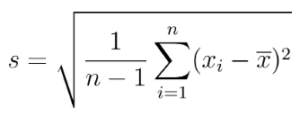
s · Sample standard deviation.
n · Sample size.
xi · Observations of the sample.
x̄ · Sample mean.
For example, considering the hourly sample of previous price variations (in pips) we have the following results:
| n | 24 |
| x̄ | 12,71 |
| ∑(xᵢ – x̄)² | 63771,96 |
And the standard deviation is: 52.66 pips ($0.0005266).
According to the empirical rule and approximately, in a normal distribution:
68% of the observations are within one standard deviation of the mean.
95% of the observations are within two standard deviations of the mean.
99.7% of the observations are within three standard deviations of the mean.
Now let’s imagine that we are interested in knowing the price movement of the EURUSD in a month if current conditions continue.
To transfer the standard deviation from one period to another we use the square root of the period.
For example, if the hourly variation that we have calculated has a deviation of 52.66 pips and we want to calculate what it could have on a monthly basis, we multiply by a factor that corresponds to the square root of the hours in a month.
Assuming a month of 30 days and four weeks, knowing that the EURUSD will have worked on 5 business days, we have that a month will have (30 – 4*2) * 24 = 528 hours. Therefore:
![]()
Therefore, in one more day the possibility that the EURUSD will remain between the following values: 1.08421 ± 0.01210 is 68%.
As we see, using the normal distribution as an approximation of the movement of price variation is very useful for making assumptions.
We must take into account that I have assumed that the average price variation of the EURUSD is equal to or very close to zero. This implies that we consider its movement as random (stochastic).
The Lognormal distribution and volatility
If we consider that the movement of prices approaches a lognormal distribution (rather than a normal distribution) we can deduce that the variation of the natural logarithm of prices follows a normal distribution.
Therefore, if in the previous section we started from the difference in prices to calculate the standard deviation, now we will start from the difference in the natural logarithms of prices to calculate the standard deviation.
Let’s continue with the previous example:
| Hour | Ask | Bid | Price | Ln Price | Variation in hours |
| 1:00:00 | 1,08117 | 1,08115 | 1,08116 | 0,07803 | 0 |
| 2:00:00 | 1,08215 | 1,08212 | 1,08214 | 0,07894 | 0,00090 |
| 3:00:00 | 1,08187 | 1,08184 | 1,08186 | 0,07868 | -0,00026 |
| 4:00:00 | 1,08171 | 1,08170 | 1,08171 | 0,07854 | -0,00014 |
| 5:00:00 | 1,08140 | 1,08137 | 1,08139 | 0,07824 | -0,00030 |
| 6:00:00 | 1,08124 | 1,08122 | 1,08123 | 0,07810 | -0,00014 |
| 7:00:00 | 1,08091 | 1,08091 | 1,08091 | 0,07780 | -0,00030 |
| 8:00:00 | 1,08127 | 1,08126 | 1,08127 | 0,07813 | 0,00033 |
| 9:00:00 | 1,08112 | 1,08110 | 1,08111 | 0,07799 | -0,00014 |
| 10:00:00 | 1,08162 | 1,08156 | 1,08159 | 0,07843 | 0,00044 |
| 11:00:00 | 1,08108 | 1,08105 | 1,08107 | 0,07795 | -0,00049 |
| 12:00:00 | 1,08189 | 1,08187 | 1,08188 | 0,07870 | 0,00075 |
| 13:00:00 | 1,08132 | 1,08129 | 1,08131 | 0,07817 | -0,00053 |
| 14:00:00 | 1,08129 | 1,08127 | 1,08128 | 0,07815 | -0,00002 |
| 15:00:00 | 1,08221 | 1,08199 | 1,08210 | 0,07890 | 0,00076 |
| 16:00:00 | 1,08356 | 1,08354 | 1,08355 | 0,08024 | 0,00134 |
| 17:00:00 | 1,08308 | 1,08306 | 1,08307 | 0,07980 | -0,00044 |
| 18:00:00 | 1,08379 | 1,08376 | 1,08378 | 0,08045 | 0,00065 |
| 19:00:00 | 1,08408 | 1,08406 | 1,08407 | 0,08072 | 0,00027 |
| 20:00:00 | 1,08415 | 1,08412 | 1,08414 | 0,08078 | 0,00006 |
| 21:00:00 | 1,08374 | 1,08373 | 1,08374 | 0,08041 | -0,00037 |
| 22:00:00 | 1,08408 | 1,08372 | 1,08390 | 0,08057 | 0,00015 |
| 23:00:00 | 1,08407 | 1,08395 | 1,08401 | 0,08067 | 0,00010 |
| 0:00:00 | 1,08421 | 1,08421 | 1,08421 | 0,08085 | 0,00018 |
The hourly variation is the sample observation that we will use to calculate the standard deviation.
A note, we have calculated the hourly variation from the variation of the natural logarithm of the current price and the natural logarithm of the previous price. Knowing the calculation of logarithms we can deduce that we could have calculated the variation by taking the natural logarithm of the current price divided by the previous price. And, most importantly, the result would be very similar if we had calculated it in the following way: Difference between the current price and the previous one divided by the average of the current price and the previous price.
In short, the variation that we have calculated is still a variation in price per unit (multiplying by one we would have a percentage variation in price).
Now we calculate the standard deviation using the formula we already know: 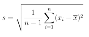
| n | 24 |
| x̄ | 0,000117378 |
| ∑(xᵢ – x̄)² | 0,000005445 |
| s horària | 0,000486555 |
| s monthly | 0,01118019203 |
The standard deviation of this distribution expressed as a percentage is known as volatility.
The hourly deviation is 0.000486555 and the monthly (multiplying by the root of 528) is 0.01118. Therefore, and multiplying by 100, we can say that the hourly volatility is 0.05% and the monthly, 1.12%.
Ultimately, there is a 68% chance that the price of EURUSD will have moved within the ±1.12% range by the end of this month.
There is a 95% chance that the EURUSD price will have moved within the ±2.24% range by the end of this month.
There is a 99.7% chance that the EURUSD price will have moved within the ±3.36% range by the end of this month.
When they tell us that the EURUSD has an annual volatility of 4%, we can do the opposite exercise to what we have done so far and find out what the monthly volatility would be:
Annual volatility = 4%
Monthly volatility = Annual volatility / SQR(12) = 1.15%